MultiREx - Fixed parameters exploration
Planetary transmission spectra generator
GitHub Repository
![]()
External dependencies
If you are working in Google Colab use this to install dependencies.
[1]:
import sys
if 'google.colab' in sys.modules:
    !pip install -Uq multirex
    !mkdir resources/
If you have already reset the Colab session, let’s import MultiREx and any other package required for this example:
[2]:
import os
import numpy as np
import pandas as pd
import matplotlib.pyplot as plt
from matplotlib.ticker import FuncFormatter
import multirex as mrex
Loading MultiREx version 0.1.5
Creating a Base System
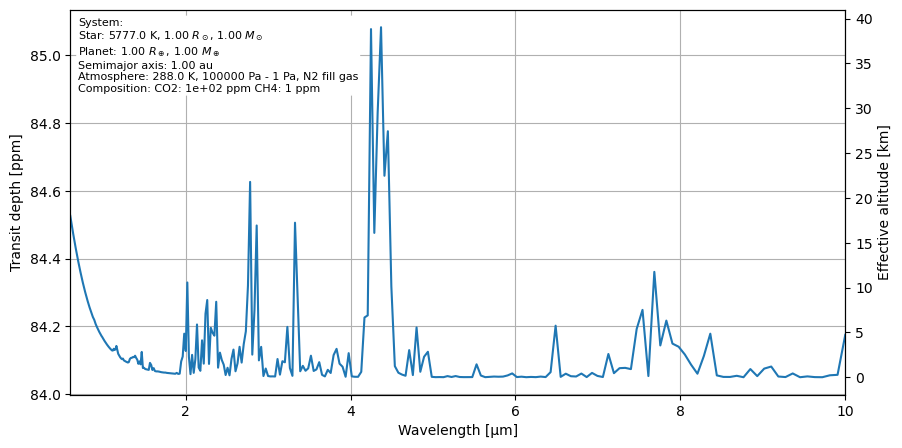
Let’s start by creating a base system.
[3]:
system = mrex.System(
    star=mrex.Star(
        temperature=5777,  # Sun-like effective temperature [K]
        radius=1,         # Solar radii
        mass=1            # Solar masses
    ),
    planet=mrex.Planet(
        radius=1,         # Earth radii
        mass=1,           # Earth masses
        atmosphere=mrex.Atmosphere(
            temperature=288,    # Earth-like temperature [K]
            base_pressure=1e5,  # Surface pressure [Pa]
            top_pressure=1,     # Top of atmosphere pressure [Pa]
            fill_gas='N2',
            composition=dict(
                CO2=-4,  # log10(mixing ratio)
                CH4=-6,  # log10(mixing ratio)
            )
        )
    ),
    sma=1  # Semi-major axis [AU]
)

system.make_tm()

wns = mrex.Physics.wavenumber_grid(wl_min=0.6, wl_max=10, resolution=300)

system.plot_spectrum(wn_grid=wns)
[3]:
(<Figure size 1000x500 with 2 Axes>,
 <Axes: xlabel='Wavelength [μm]', ylabel='Transit depth [ppm]'>)
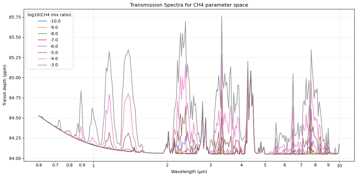
Parameter Space Exploration for a Single Molecule
This section demonstrates how to explore a molecule’s parameter space using the explore_parameter_space System method. ### Parameter Space Definition The parameter space is defined as a dictionary where:
Keys represent the parameters you want to explore
Values specify the ranges or specific values for each parameter
For example:
Star Properties
Temperature:
star.temperature(in Kelvin)
Planet Properties
Radius:
planet.radius(in Earth radii)
Atmospheric Properties
Composition:
atmosphere.composition.H2O(in volume mixing ratio)Note:
atmosphere.compositionis implemented as a dictionary of molecular species ### Parameter Value Formats Parameters can be specified in three different formats:
Single Value
-2 # Direct numerical value
List of Discrete Values
[200, 400, 1000] # Specific points to evaluate
Range Dictionary
{
    'min': 200,    # Minimum value
    'max': 1000,   # Maximum value
    'n': 10,       # Number of points
    'distribution': 'log'|'linear'  # Spacing between points
}
[!NOTE] The rest of parameters will be fixed.
[4]:
print("Exploring CH4 parameter space...")

parameter_space_ch4 = {
    'planet.atmosphere.composition.CH4': {
        'min': -10,
        'max': -3,
        'n': 8,
        'distribution': 'linear'
    }
}

results_ch4 = system.explore_parameter_space(
    wn_grid=wns,
    parameter_space=parameter_space_ch4,
    snr=20,
    n_observations=1,
    header=True  # to return a dataframe with parameters and spectra
)

spectra_ch4 = results_ch4['spectra']

# Plot spectra for different CH4 concentrations
fig_ch4, ax_ch4 = plt.subplots(figsize=(12, 6))

wavelengths = 1e4 / wns  # Convert wavenumber [cm^-1] to wavelength [μm]
ch4_values = [
    params['atm CH4']
    for _, params in spectra_ch4.params.iterrows()
]

for i, (_, spectrum) in enumerate(spectra_ch4.data.iterrows()):
    ch4_value = ch4_values[i]
    ax_ch4.plot(
        wavelengths,
        spectrum * 1e6,
        label=f'{ch4_value:.1f}',
        alpha=0.8
    )

ax_ch4.set_xscale('log')
ax_ch4.set_xlabel('Wavelength (μm)')
ax_ch4.set_ylabel('Transit depth (ppm)')
ax_ch4.set_title('Transmission Spectra for CH4 parameter space')
ax_ch4.legend(title='log10(CH4 mix ratio)')
ax_ch4.grid(True, alpha=0.3)

formatter = FuncFormatter(lambda y, _: '{:.16g}'.format(y))
ax_ch4.xaxis.set_major_formatter(formatter)
formatter = FuncFormatter(lambda y, _: '{:.1g}'.format(y))
ax_ch4.xaxis.set_minor_formatter(formatter)

plt.tight_layout()
plt.show()
Exploring CH4 parameter space...
Generating observations for 8 spectra...
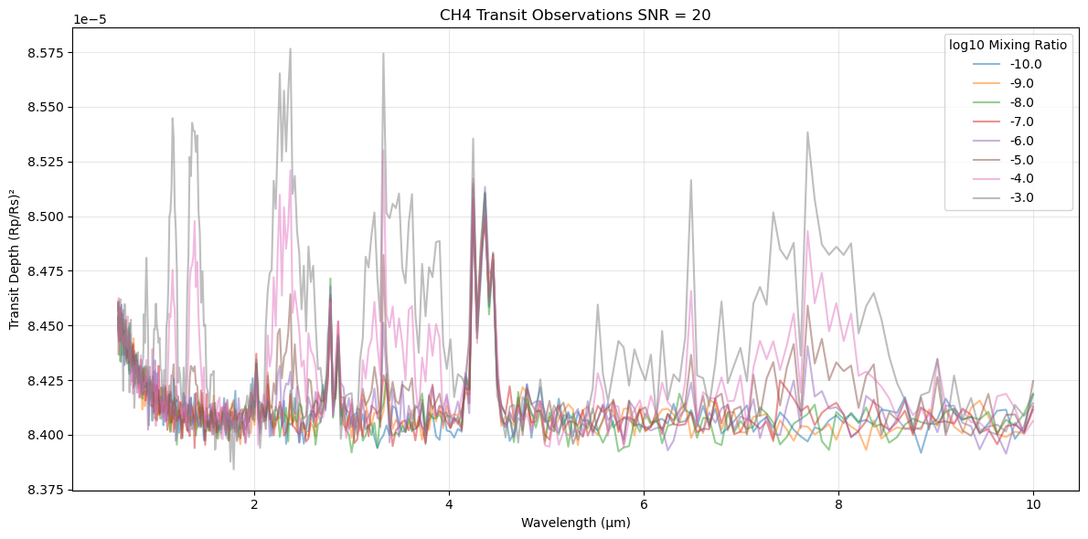
[5]:
# Display observations data
data = results_ch4["observations"].data
wavelengths = list(results_ch4["observations"].data.columns)

# Create figure and axis objects
fig, ax = plt.subplots(figsize=(12, 6))

# Plot each observation
for i in range(data.shape[0]):
    ch4_value = results_ch4["observations"]["atm CH4"][i]
    ax.plot(
        wavelengths,
        data.iloc[i],
        label=f'{ch4_value:.1f}',
        alpha=0.5
    )

# Customize plot appearance
ax.set_xlabel('Wavelength (μm)')
ax.set_ylabel('Transit Depth (Rp/Rs)²')
ax.set_title('CH4 Transit Observations SNR = 20')
ax.legend(title='log10 Mixing Ratio')
ax.grid(True, alpha=0.3)

# Adjust layout to prevent label clipping
plt.tight_layout()
plt.show()
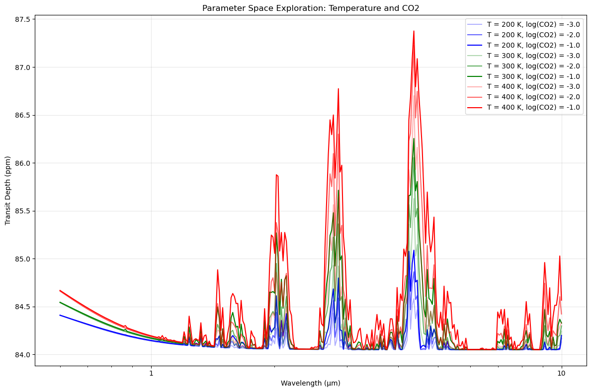
Parameter exploration with various MultiREx components
You can explore various parameters in the system, obtaining a combination between each of them at the end.
[6]:
print("Exploring temperature and CO2 parameter space...")


PARAMETER_SPACE_TEMP_CO2 = {
    'planet.atmosphere.temperature': [200, 300, 400],  # List of temperatures
    'planet.atmosphere.composition.CO2': {  # Dictionary for CO2 mixing ratio
        'min': -3,  # Minimum log10(mixing ratio)
        'max': -1,  # Maximum log10(mixing ratio)
        'n': 3,
        'distribution': 'linear'
    }
}

if system.get_params().get("atm CH4"):
    system.planet.atmosphere.remove_gas("CH4")

results_temp_co2 = system.explore_parameter_space(
    wn_grid=wns,
    parameter_space=PARAMETER_SPACE_TEMP_CO2,
    snr=20,
    n_observations=1,
    header=True
)

spectra_temp_co2 = results_temp_co2['spectra']

# Create figure and axis objects
fig, ax = plt.subplots(figsize=(12, 8))

# Plot spectra with temperature-based coloring
COLORS = ['b', 'g', 'r']
temperatures = sorted(spectra_temp_co2.params['atm temperature'].unique())
color_dict = dict(zip(temperatures, COLORS))
ALPHAS = [0.3, 0.6, 1]

for idx, (_, params) in enumerate(spectra_temp_co2.params.iterrows()):
    temp = params['atm temperature']
    co2_value = params['atm CO2']
    spectrum = spectra_temp_co2.data.loc[idx]

    ax.plot(
        wavelengths,
        spectrum * 1e6,
        label=f'T = {temp:.0f} K, log(CO2) = {co2_value:.1f}',
        color=color_dict[temp],
        alpha=ALPHAS[idx % 3]
    )

# Customize plot appearance
ax.set_xscale('log')
ax.set_ylabel('Transit Depth (ppm)')
ax.set_xlabel('Wavelength (μm)')
ax.set_title('Parameter Space Exploration: Temperature and CO2')
ax.legend()
ax.grid(True, alpha=0.3)

# Format axes
ax.xaxis.set_major_formatter(FuncFormatter(lambda y, _: '{:.16g}'.format(y)))

plt.tight_layout()
plt.show()
Exploring temperature and CO2 parameter space...
c:\Users\User\anaconda3\Lib\site-packages\taurex\data\profiles\pressure\pressureprofile.py:137: DeprecationWarning: SimplePressureProfile is deprecated. Use LogPressureProfile instead
  warn(
c:\Users\User\anaconda3\Lib\site-packages\taurex\model\transmission.py:80: DeprecationWarning: SimpleForwardModel is deprecated. Use OneDForwardModel instead
  super().__init__(
c:\Users\User\anaconda3\Lib\site-packages\taurex\data\planet.py:136: DeprecationWarning: fullRadius is deprecated, use get_planet_radius(unit='m') instead
  warn(
Generating observations for 9 spectra...
Parallel Processing
Since generating spectra across the entire parameter space quickly scales with the number of parameters, MultiREx allows parallel exploration of the parameter space. To achieve this, you only need to specify the number of processors to use with the n_jobs parameter in the explore_parameter_space function.
[10]:
import time

system.planet.atmosphere.set_composition({
    "CO2": -2,
    "CH4": -1,
    "H2O": -1
})

parameter_space_parallel = {
    "planet.atmosphere.composition.CO2": {
        "min": -10,
        "max": -1,
        "n": 10
    },
    "planet.atmosphere.composition.H2O": {
        "min": -10,
        "max": -1,
        "n": 10
    },
    "planet.atmosphere.composition.CH4": {
        "min": -10,
        "max": -1,
        "n": 10
    }
}

start_time = time.time()
results = system.explore_parameter_space(
    wn_grid=wns,
    parameter_space=parameter_space_parallel,
    snr=20,
    n_observations=1000,
    header=True,
    n_jobs=-1
)

parallel_time = time.time() - start_time
results['spectra'].params.describe()
Generating observations for 1000 spectra...
[10]:
| sma | seed | p_radius | p_mass | p_seed | atm temperature | atm base_pressure | atm top_pressure | atm seed | atm CO2 | atm CH4 | atm H2O | s temperature | s radius | s mass | s seed | |
|---|---|---|---|---|---|---|---|---|---|---|---|---|---|---|---|---|
| count | 1000.0 | 1.000000e+03 | 1000.0 | 1000.0 | 1.000000e+03 | 1000.0 | 1000.0 | 1000.0 | 1.000000e+03 | 1000.000000 | 1000.000000 | 1000.000000 | 1000.0 | 1000.0 | 1000.0 | 1.000000e+03 |
| mean | 1.0 | 1.742360e+09 | 1.0 | 1.0 | 1.742360e+09 | 288.0 | 100000.0 | 1.0 | 1.742360e+09 | -5.500000 | -5.500000 | -5.500000 | 5777.0 | 1.0 | 1.0 | 1.742360e+09 |
| std | 0.0 | 0.000000e+00 | 0.0 | 0.0 | 0.000000e+00 | 0.0 | 0.0 | 0.0 | 0.000000e+00 | 2.873719 | 2.873719 | 2.873719 | 0.0 | 0.0 | 0.0 | 0.000000e+00 |
| min | 1.0 | 1.742360e+09 | 1.0 | 1.0 | 1.742360e+09 | 288.0 | 100000.0 | 1.0 | 1.742360e+09 | -10.000000 | -10.000000 | -10.000000 | 5777.0 | 1.0 | 1.0 | 1.742360e+09 |
| 25% | 1.0 | 1.742360e+09 | 1.0 | 1.0 | 1.742360e+09 | 288.0 | 100000.0 | 1.0 | 1.742360e+09 | -8.000000 | -8.000000 | -8.000000 | 5777.0 | 1.0 | 1.0 | 1.742360e+09 |
| 50% | 1.0 | 1.742360e+09 | 1.0 | 1.0 | 1.742360e+09 | 288.0 | 100000.0 | 1.0 | 1.742360e+09 | -5.500000 | -5.500000 | -5.500000 | 5777.0 | 1.0 | 1.0 | 1.742360e+09 |
| 75% | 1.0 | 1.742360e+09 | 1.0 | 1.0 | 1.742360e+09 | 288.0 | 100000.0 | 1.0 | 1.742360e+09 | -3.000000 | -3.000000 | -3.000000 | 5777.0 | 1.0 | 1.0 | 1.742360e+09 |
| max | 1.0 | 1.742360e+09 | 1.0 | 1.0 | 1.742360e+09 | 288.0 | 100000.0 | 1.0 | 1.742360e+09 | -1.000000 | -1.000000 | -1.000000 | 5777.0 | 1.0 | 1.0 | 1.742360e+09 |
[9]:
t = time.time()
results = system.explore_parameter_space(
    wn_grid=wns,
    parameter_space=parameter_space_parallel,
    snr=20,
    n_observations=1000,
    header=True,
    n_jobs = 1,
)
sequential_time = time.time() - t
c:\Users\User\anaconda3\Lib\site-packages\taurex\data\profiles\pressure\pressureprofile.py:137: DeprecationWarning: SimplePressureProfile is deprecated. Use LogPressureProfile instead
  warn(
c:\Users\User\anaconda3\Lib\site-packages\taurex\model\transmission.py:80: DeprecationWarning: SimpleForwardModel is deprecated. Use OneDForwardModel instead
  super().__init__(
c:\Users\User\anaconda3\Lib\site-packages\taurex\data\planet.py:136: DeprecationWarning: fullRadius is deprecated, use get_planet_radius(unit='m') instead
  warn(
Generating observations for 1000 spectra...
[11]:
print("Total number of spectra: ", len(results["spectra"]))

# Create DataFrames with value counts for spectra
spectra_ch4 = results["spectra"].params[["atm CH4"]].value_counts()
spectra_co2 = results["spectra"].params[["atm CO2"]].value_counts()
spectra_h2o = results["spectra"].params[["atm H2O"]].value_counts()

# Combine into a single DataFrame for spectra
spectra_counts = pd.concat([spectra_ch4, spectra_co2, spectra_h2o], axis=1)
spectra_counts.columns = ['CH4', 'CO2', 'H2O']
print("\nSpectra parameter counts:")
print(spectra_counts)

print("\n" + "----"*10)

print("\nTotal number of observations: ", len(results["observations"]))

# Create DataFrames with value counts for observations
obs_ch4 = results["observations"].params[["atm CH4"]].value_counts()
obs_co2 = results["observations"].params[["atm CO2"]].value_counts()
obs_h2o = results["observations"].params[["atm H2O"]].value_counts()

# Combine into a single DataFrame for observations
obs_counts = pd.concat([obs_ch4, obs_co2, obs_h2o], axis=1)
obs_counts.columns = ['CH4', 'CO2', 'H2O']
print("\nObservation parameter counts:")
print(obs_counts)

print("\n" + "----"*10)
print(f"Time taken:\nSequential: {sequential_time}\nParallel: {parallel_time}")
Total number of spectra:  1000

Spectra parameter counts:
       CH4  CO2  H2O
-10.0  100  100  100
-9.0   100  100  100
-8.0   100  100  100
-7.0   100  100  100
-6.0   100  100  100
-5.0   100  100  100
-4.0   100  100  100
-3.0   100  100  100
-2.0   100  100  100
-1.0   100  100  100

----------------------------------------

Total number of observations:  1000000

Observation parameter counts:
          CH4     CO2     H2O
-10.0  100000  100000  100000
-9.0   100000  100000  100000
-8.0   100000  100000  100000
-7.0   100000  100000  100000
-6.0   100000  100000  100000
-5.0   100000  100000  100000
-4.0   100000  100000  100000
-3.0   100000  100000  100000
-2.0   100000  100000  100000
-1.0   100000  100000  100000

----------------------------------------
Time taken:
Sequential: 87.17826914787292
Parallel: 23.5948007106781
[ ]: