MultiREx - Quickstart
Planetary transmission spectra generator
GitHub Repository
![]()
External dependencies
If you are working in Google Colab use this to install dependencies.
[38]:
import sys
if 'google.colab' in sys.modules:
    !pip install -Uq multirex
    !mkdir resources/
NOTE: After installing you should reset Colab session before importing the package. This is to avoid an unintended behavior of the package
pybtex.
If you have already reset the Colab session, let’s import MultiREx and any other package required for this example:
[2]:
import multirex as mrex
import numpy as np
import matplotlib.pyplot as plt
import pandas as pd
# This is for developing purposes
%load_ext autoreload
%autoreload 2
Loading MultiREx version 0.1.5
Creating a single system
Components
The central concept in MultiREx is that of a system. A system is made of a star, a planet and its atmosphere. Each component may have a wide range of properties useful for the purposes of the package. However, the key properties required for calculating a basic transmission spectra are defined below:
Star:
Effective temperature in Kelvins (attribute
temperature).Radius in solar radii (attribute
radius).Mass in solar masses (attribute
mass).
Planet:
Radius in Earth radii (attribute
radius).Mass in Earth masses (attribute
mass).
Atmosphere:
Surface temperature in Kelvins (attribute
temperature).Surface pressure in Pascals (attribute
base_pressure).Pressure at the top of the atmosphere in Pascals (attribute
top_pressure).Composition (attribute
composition). This is provided as a dictionary whose keys are the name of the gasses (e.g. ‘CO2’, ‘CH4’) and the value are the \(log_{10}\) of the mixing ratio of the corresponding gas.Fill gass name (attribute
fill_gass), i.e. the gass which fills the atmopshere (usually ‘N2’ for atmospheres of inhabited planets).
Available gasses
If you want to see the list of available gasses in the package use:
[3]:
mrex.Util.list_gases()
Available gases in the database:
['CO2', 'CH4', 'O2', 'O3', 'H2O']
MultiREx comes along with ExoTransmit opacities for these particular gasses. These opacities are low resolution and light-weighted. They should be used only for testing purposes. For larger scientific applications, MultiREx provides a larger database of high-resolution opacities (most of them from ExoMol) for a larger number of gasses. This database is hosted in a Google Drive
repository and can be obtained and loaded into the running instance of MultiREx using:
WARNING: Be careful with this command: it will use as much as 4 GB of disk space.
[39]:
mrex.Util.get_gases(path='/tmp')
The directory to the opacity database already exists in the specified path: /tmp
Once downloaded, the list of available gasses are considerably larger:_
[5]:
mrex.Util.list_gases()
Available gases in the database:
['DMS', 'NO2', 'SO2', 'CO', 'CO2', 'CH4', 'NH3', 'HCN', 'O2', 'O3', 'C2H6', 'CH3Cl', 'H2O', 'N2']
Creating components of the system
Let’s create a star:
[6]:
star = mrex.Star(temperature=5777,radius=1,mass=1)
You may get the attributes of the star using:
[7]:
star.mass, star.temperature
[7]:
(1, 5777)
You may also modify the mass of the star:
[8]:
star.set_mass(1.5)
Now create the planet:
[9]:
planet = mrex.Planet(radius=1,mass=1)
And finally create the atmosphere:
[10]:
atmosphere = mrex.Atmosphere(
    temperature=288, # in K
    base_pressure=1e5, # in Pa
    top_pressure=1, # in Pa
    fill_gas='N2', # the gas that fills the atmosphere
    composition=dict(
        CO2=-4, # This is the log10(mix-ratio)
        CH4=-6,
    )
)
Once created we can integrate the three components in a system:
[11]:
planet.set_atmosphere(atmosphere)
system = mrex.System(star=star,planet=planet,sma=1)
After ensembling the components you still have access to the properties independently:
[12]:
system.planet.radius
[12]:
1
We can ensemble a system using a single command like:
[13]:
system = mrex.System(
    star=mrex.Star(
        temperature=5777,
        radius=1,
        mass=1
    ),
    planet=mrex.Planet(
        radius=1,
        mass=1,
        atmosphere=mrex.Atmosphere(
            temperature=290, # in K
            base_pressure=1e5, # in Pa
            top_pressure=1, # in Pa
            fill_gas='N2', # the gas that fills the atmosphere
            composition=dict(
                CO2=-4, # This is the log10(mix-ratio)
                CH4=-6,
            )
        )
    ),
    sma=1
)
The transmission model
Once we have a system we can create the transmission model:
[14]:
system.make_tm()
The transmission model is a Taurex class that allows us to create transmission spectra as desired. It encapsulates all the attributes and methods used to described the atmosphere that are taken into account when calculating the transmission spectra. MultiREx essentially simplify the interaction with the wide range of options of TauREx for specifying those attributes.
You may take a quick look to the attributes of the transmission model using:
[15]:
system.transmission.__dict__
[15]:
{'_log_name': 'taurex.TransmissionModel',
 '_logger': <Logger taurex.TransmissionModel (ERROR)>,
 '_param_dict': {},
 '_derived_dict': {},
 'opacity_dict': {},
 'cia_dict': {},
 '_native_grid': None,
 '_derived_parameters': {'logg': ('logg',
   'log(g)',
   <bound method derivedparam.<locals>.wrapper of <taurex.data.planet.Planet object at 0x7f365fab35b0>>,
   False),
  'avg_T': ('avg_T',
   '$\\bar{T}$',
   <bound method derivedparam.<locals>.wrapper of <taurex.data.profiles.temperature.isothermal.Isothermal object at 0x7f365fab3a30>>,
   False),
  'metallicity': ('metallicity',
   'Z',
   <bound method derivedparam.<locals>.wrapper of <taurex.data.profiles.chemistry.taurexchemistry.TaurexChemistry object at 0x7f365fab39a0>>,
   False),
  'mu': ('mu',
   '$\\mu$',
   <bound method derivedparam.<locals>.wrapper of <taurex.data.profiles.chemistry.taurexchemistry.TaurexChemistry object at 0x7f365fab39a0>>,
   True)},
 '_fitting_parameters': {'planet_mass': ('planet_mass',
   '$M_p$',
   <bound method fitparam.<locals>.wrapper of <taurex.data.planet.Planet object at 0x7f365fab35b0>>,
   <bound method BasePlanet.mass of <taurex.data.planet.Planet object at 0x7f365fab35b0>>,
   'linear',
   False,
   [0.5, 1.5]),
  'planet_radius': ('planet_radius',
   '$R_p$',
   <bound method fitparam.<locals>.wrapper of <taurex.data.planet.Planet object at 0x7f365fab35b0>>,
   <bound method BasePlanet.radius of <taurex.data.planet.Planet object at 0x7f365fab35b0>>,
   'linear',
   True,
   [0.9, 1.1]),
  'planet_distance': ('planet_distance',
   '$D_{planet}$',
   <bound method fitparam.<locals>.wrapper of <taurex.data.planet.Planet object at 0x7f365fab35b0>>,
   <bound method BasePlanet.distance of <taurex.data.planet.Planet object at 0x7f365fab35b0>>,
   'linear',
   False,
   [1, 2]),
  'planet_sma': ('planet_sma',
   '$D_{planet}$',
   <bound method fitparam.<locals>.wrapper of <taurex.data.planet.Planet object at 0x7f365fab35b0>>,
   <bound method BasePlanet.semiMajorAxis of <taurex.data.planet.Planet object at 0x7f365fab35b0>>,
   'linear',
   False,
   [1, 2]),
  'atm_min_pressure': ('atm_min_pressure',
   '$P_\\mathrm{min}$',
   <bound method fitparam.<locals>.wrapper of <taurex.data.profiles.pressure.pressureprofile.SimplePressureProfile object at 0x7f365fab3d90>>,
   <bound method SimplePressureProfile.minAtmospherePressure of <taurex.data.profiles.pressure.pressureprofile.SimplePressureProfile object at 0x7f365fab3d90>>,
   'log',
   False,
   [0.1, 1.0]),
  'atm_max_pressure': ('atm_max_pressure',
   '$P_\\mathrm{max}$',
   <bound method fitparam.<locals>.wrapper of <taurex.data.profiles.pressure.pressureprofile.SimplePressureProfile object at 0x7f365fab3d90>>,
   <bound method SimplePressureProfile.maxAtmospherePressure of <taurex.data.profiles.pressure.pressureprofile.SimplePressureProfile object at 0x7f365fab3d90>>,
   'log',
   False,
   [0.1, 1.0]),
  'T': ('T',
   '$T$',
   <bound method fitparam.<locals>.wrapper of <taurex.data.profiles.temperature.isothermal.Isothermal object at 0x7f365fab3a30>>,
   <bound method Isothermal.isoTemperature of <taurex.data.profiles.temperature.isothermal.Isothermal object at 0x7f365fab3a30>>,
   'linear',
   False,
   [300.0, 2000.0]),
  'CO2': ('CO2',
   'CO$_2$',
   <bound method ConstantGas.add_active_gas_param.<locals>.read_mol of <taurex.data.profiles.chemistry.gas.constantgas.ConstantGas object at 0x7f365fab3970>>,
   <bound method ConstantGas.add_active_gas_param.<locals>.write_mol of <taurex.data.profiles.chemistry.gas.constantgas.ConstantGas object at 0x7f365fab3970>>,
   'log',
   False,
   [1e-12, 0.1]),
  'CH4': ('CH4',
   'CH$_4$',
   <bound method ConstantGas.add_active_gas_param.<locals>.read_mol of <taurex.data.profiles.chemistry.gas.constantgas.ConstantGas object at 0x7f365fab3940>>,
   <bound method ConstantGas.add_active_gas_param.<locals>.write_mol of <taurex.data.profiles.chemistry.gas.constantgas.ConstantGas object at 0x7f365fab3940>>,
   'log',
   False,
   [1e-12, 0.1])},
 'contribution_list': [<taurex.contributions.absorption.AbsorptionContribution at 0x7f365fab3f10>,
  <taurex.contributions.rayleigh.RayleighContribution at 0x7f365fab2bc0>],
 '_planet': <taurex.data.planet.Planet at 0x7f365fab35b0>,
 '_star': <taurex.data.stellar.star.BlackbodyStar at 0x7f365fab3e50>,
 '_pressure_profile': <taurex.data.profiles.pressure.pressureprofile.SimplePressureProfile at 0x7f365fab3d90>,
 '_temperature_profile': <taurex.data.profiles.temperature.isothermal.Isothermal at 0x7f365fab3a30>,
 '_chemistry': <taurex.data.profiles.chemistry.taurexchemistry.TaurexChemistry at 0x7f365fab39a0>,
 'altitude_profile': array([     0.        ,   1011.27930182,   2022.87931573,   3034.80019431,
          4047.04209025,   5059.60515631,   6072.48954536,   7085.69541037,
          8099.22290441,   9113.07218063,  10127.2433923 ,  11141.73669277,
         12156.5522355 ,  13171.69017404,  14187.15066203,  15202.93385322,
         16219.03990146,  17235.46896068,  18252.22118493,  19269.29672835,
         20286.69574517,  21304.41838973,  22322.46481645,  23340.83517987,
         24359.52963461,  25378.54833541,  26397.89143709,  27417.55909457,
         28437.55146287,  29457.86869713,  30478.51095255,  31499.47838445,
         32520.77114827,  33542.3893995 ,  34564.33329378,  35586.60298681,
         36609.19863441,  37632.12039249,  38655.36841707,  39678.94286426,
         40702.84389028,  41727.07165144,  42751.62630414,  43776.5080049 ,
         44801.71691034,  45827.25317716,  46853.11696219,  47879.30842232,
         48905.82771457,  49932.67499607,  50959.85042401,  51987.35415571,
         53015.18634859,  54043.34716017,  55071.83674806,  56100.65526997,
         57129.80288372,  58159.27974723,  59189.08601853,  60219.22185573,
         61249.68741705,  62280.48286082,  63311.60834546,  64343.06402949,
         65374.85007155,  66406.96663037,  67439.41386477,  68472.19193369,
         69505.30099616,  70538.74121132,  71572.51273841,  72606.61573677,
         73641.05036583,  74675.81678515,  75710.91515438,  76746.34563326,
         77782.10838164,  78818.20355948,  79854.63132685,  80891.39184389,
         81928.48527087,  82965.91176816,  84003.67149622,  85041.76461564,
         86080.19128708,  87118.95167132,  88158.04592925,  89197.47422185,
         90237.23671022,  91277.33355553,  92317.76491909,  93358.53096231,
         94399.63184667,  95441.0677338 ,  96482.8387854 ,  97524.94516328,
         98567.38702938,  99610.16454571, 100653.2778744 , 101696.72717769]),
 'scaleheight_profile': array([8783.86040885, 8786.6460787 , 8789.43307384, 8792.22139511,
        8795.01104336, 8797.80201942, 8800.59432413, 8803.38795835,
        8806.18292292, 8808.97921867, 8811.77684646, 8814.57580713,
        8817.37610152, 8820.1777305 , 8822.9806949 , 8825.78499557,
        8828.59063336, 8831.39760912, 8834.20592371, 8837.01557797,
        8839.82657276, 8842.63890893, 8845.45258733, 8848.26760882,
        8851.08397426, 8853.90168449, 8856.72074037, 8859.54114277,
        8862.36289254, 8865.18599053, 8868.01043761, 8870.83623463,
        8873.66338247, 8876.49188196, 8879.32173399, 8882.15293941,
        8884.98549909, 8887.81941388, 8890.65468466, 8893.49131228,
        8896.32929762, 8899.16864154, 8902.00934491, 8904.8514086 ,
        8907.69483347, 8910.53962039, 8913.38577023, 8916.23328388,
        8919.08216218, 8921.93240603, 8924.78401629, 8927.63699383,
        8930.49133953, 8933.34705426, 8936.20413891, 8939.06259434,
        8941.92242143, 8944.78362106, 8947.64619411, 8950.51014146,
        8953.37546399, 8956.24216258, 8959.1102381 , 8961.97969145,
        8964.8505235 , 8967.72273514, 8970.59632725, 8973.47130071,
        8976.34765642, 8979.22539526, 8982.10451811, 8984.98502586,
        8987.8669194 , 8990.75019963, 8993.63486742, 8996.52092368,
        8999.40836928, 9002.29720513, 9005.18743211, 9008.07905112,
        9010.97206306, 9013.86646881, 9016.76226928, 9019.65946536,
        9022.55805794, 9025.45804793, 9028.35943621, 9031.26222371,
        9034.1664113 , 9037.07199989, 9039.97899039, 9042.88738369,
        9045.7971807 , 9048.70838232, 9051.62098945, 9054.53500301,
        9057.45042389, 9060.36725301, 9063.28549126]),
 'gravity_profile': array([9.79839813, 9.7952917 , 9.79218577, 9.78908032, 9.78597537,
        9.78287091, 9.77976694, 9.77666347, 9.77356048, 9.770458  ,
        9.767356  , 9.76425449, 9.76115348, 9.75805296, 9.75495294,
        9.7518534 , 9.74875436, 9.74565581, 9.74255776, 9.73946019,
        9.73636312, 9.73326654, 9.73017046, 9.72707486, 9.72397976,
        9.72088515, 9.71779104, 9.71469741, 9.71160428, 9.70851165,
        9.7054195 , 9.70232785, 9.69923669, 9.69614602, 9.69305585,
        9.68996616, 9.68687697, 9.68378828, 9.68070007, 9.67761236,
        9.67452514, 9.67143841, 9.66835218, 9.66526644, 9.66218119,
        9.65909643, 9.65601217, 9.65292839, 9.64984512, 9.64676233,
        9.64368004, 9.64059823, 9.63751693, 9.63443611, 9.63135579,
        9.62827595, 9.62519662, 9.62211777, 9.61903942, 9.61596156,
        9.61288419, 9.60980731, 9.60673093, 9.60365504, 9.60057964,
        9.59750474, 9.59443033, 9.59135641, 9.58828298, 9.58521004,
        9.5821376 , 9.57906565, 9.57599419, 9.57292323, 9.56985276,
        9.56678278, 9.56371329, 9.5606443 , 9.5575758 , 9.55450779,
        9.55144027, 9.54837325, 9.54530671, 9.54224068, 9.53917513,
        9.53611008, 9.53304552, 9.52998145, 9.52691787, 9.52385479,
        9.5207922 , 9.5177301 , 9.51466849, 9.51160738, 9.50854676,
        9.50548663, 9.502427  , 9.49936785, 9.4963092 ]),
 '_initialized': True,
 '_sigma_opacities': None,
 'new_method': False,
 '_inital_mu': <taurex.data.profiles.chemistry.taurexchemistry.TaurexChemistry at 0x7f365fab27a0>,
 'altitude_boundaries': array([     0.        ,   1011.27930182,   2022.87931573,   3034.80019431,
          4047.04209025,   5059.60515631,   6072.48954536,   7085.69541037,
          8099.22290441,   9113.07218063,  10127.2433923 ,  11141.73669277,
         12156.5522355 ,  13171.69017404,  14187.15066203,  15202.93385322,
         16219.03990146,  17235.46896068,  18252.22118493,  19269.29672835,
         20286.69574517,  21304.41838973,  22322.46481645,  23340.83517987,
         24359.52963461,  25378.54833541,  26397.89143709,  27417.55909457,
         28437.55146287,  29457.86869713,  30478.51095255,  31499.47838445,
         32520.77114827,  33542.3893995 ,  34564.33329378,  35586.60298681,
         36609.19863441,  37632.12039249,  38655.36841707,  39678.94286426,
         40702.84389028,  41727.07165144,  42751.62630414,  43776.5080049 ,
         44801.71691034,  45827.25317716,  46853.11696219,  47879.30842232,
         48905.82771457,  49932.67499607,  50959.85042401,  51987.35415571,
         53015.18634859,  54043.34716017,  55071.83674806,  56100.65526997,
         57129.80288372,  58159.27974723,  59189.08601853,  60219.22185573,
         61249.68741705,  62280.48286082,  63311.60834546,  64343.06402949,
         65374.85007155,  66406.96663037,  67439.41386477,  68472.19193369,
         69505.30099616,  70538.74121132,  71572.51273841,  72606.61573677,
         73641.05036583,  74675.81678515,  75710.91515438,  76746.34563326,
         77782.10838164,  78818.20355948,  79854.63132685,  80891.39184389,
         81928.48527087,  82965.91176816,  84003.67149622,  85041.76461564,
         86080.19128708,  87118.95167132,  88158.04592925,  89197.47422185,
         90237.23671022,  91277.33355553,  92317.76491909,  93358.53096231,
         94399.63184667,  95441.0677338 ,  96482.8387854 ,  97524.94516328,
         98567.38702938,  99610.16454571, 100653.2778744 , 101696.72717769,
        102740.5126179 ]),
 'deltaz': array([1011.27930182, 1011.60001391, 1011.92087858, 1012.24189593,
        1012.56306606, 1012.88438905, 1013.20586501, 1013.52749404,
        1013.84927622, 1014.17121167, 1014.49330047, 1014.81554273,
        1015.13793853, 1015.46048799, 1015.78319119, 1016.10604824,
        1016.42905923, 1016.75222425, 1017.07554342, 1017.39901682,
        1017.72264455, 1018.04642672, 1018.37036342, 1018.69445475,
        1019.0187008 , 1019.34310168, 1019.66765748, 1019.99236831,
        1020.31723425, 1020.64225542, 1020.96743191, 1021.29276381,
        1021.61825124, 1021.94389427, 1022.26969303, 1022.5956476 ,
        1022.92175808, 1023.24802458, 1023.57444719, 1023.90102602,
        1024.22776115, 1024.5546527 , 1024.88170076, 1025.20890544,
        1025.53626682, 1025.86378502, 1026.19146013, 1026.51929226,
        1026.84728149, 1027.17542794, 1027.5037317 , 1027.83219288,
        1028.16081158, 1028.48958788, 1028.81852191, 1029.14761375,
        1029.47686351, 1029.8062713 , 1030.1358372 , 1030.46556132,
        1030.79544377, 1031.12548464, 1031.45568404, 1031.78604206,
        1032.11655882, 1032.4472344 , 1032.77806892, 1033.10906247,
        1033.44021516, 1033.77152709, 1034.10299836, 1034.43462907,
        1034.76641932, 1035.09836922, 1035.43047888, 1035.76274838,
        1036.09517784, 1036.42776736, 1036.76051704, 1037.09342698,
        1037.42649729, 1037.75972807, 1038.09311942, 1038.42667144,
        1038.76038424, 1039.09425793, 1039.4282926 , 1039.76248836,
        1040.09684531, 1040.43136356, 1040.76604321, 1041.10088437,
        1041.43588713, 1041.7710516 , 1042.10637789, 1042.4418661 ,
        1042.77751633, 1043.11332869, 1043.44930329, 1043.78544022])}
Generating a transmission spectrum
In order to create and manipulate a transmission spectrum, we need first to genereta a wave number grid:
[16]:
wns = mrex.Physics.wavenumber_grid(wl_min=0.6,wl_max=10,resolution=1000)
The corresponding wavelength grid is:
[17]:
wls = np.sort(1e4/wns)
wls[:10],wls[-10:]
[17]:
(array([0.6       , 0.60169212, 0.60338901, 0.60509068, 0.60679716,
        0.60850844, 0.61022456, 0.61194551, 0.61367132, 0.61540199]),
 array([ 9.74972472,  9.77722085,  9.80479454,  9.83244598,  9.86017541,
         9.88798304,  9.91586909,  9.94383379,  9.97187735, 10.        ]))
Let’s generate the transmission spectrum:
[18]:
wns,spectrum = system.generate_spectrum(wns)
wls = 1e4/wns
The spectrum is an adimensional quantity given in terms of the fraction of the stellar area blocked by the planet and its atmosphere, in other words \((R_p/R_\star)^2\). It is conventionally measured in parts per million (ppm) and conventionally called transit depth. In our case, if the planet was air-less it will produce a spectrum with a depth of:
[19]:
from astropy.constants import R_sun, R_earth
1e6*(system.planet.radius*R_earth/(system.star.radius*R_sun))**2
[19]:
Once the spectrum has been calculated we can plot it:
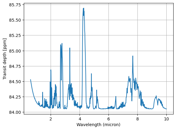
[20]:
plt.plot(wls,spectrum*1e6)
plt.grid()
plt.xlabel('Wavelength (micron)')
plt.ylabel('Transit depth [ppm]')
[20]:
Text(0, 0.5, 'Transit depth [ppm]')
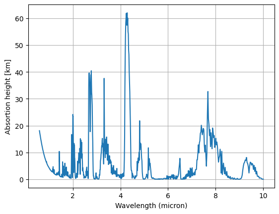
You can also plot the spectrum using the absortion height, namely the apparent size of the atmosphere as seen at a given wavelength and which is given by:
[21]:
effalts = (np.sqrt(spectrum)*system.star.radius*R_sun.value - system.planet.radius*R_earth.value)/1e3
effalts[:10]
[21]:
array([0.07626681, 0.06778101, 0.11127472, 0.37537931, 0.50011134,
       0.52420784, 0.45433174, 1.1838071 , 1.08375566, 1.17605428])
This is precisely the function of the routine mrex.Physics.spectrum2height:
[22]:
effalts = mrex.Physics.spectrum2altitude(spectrum,system.planet.radius,system.star.radius)
Let’s plot it:
[23]:
plt.plot(wls,effalts)
plt.grid()
plt.xlabel('Wavelength (micron)')
plt.ylabel('Absortion height [km]')
[23]:
Text(0, 0.5, 'Absortion height [km]')
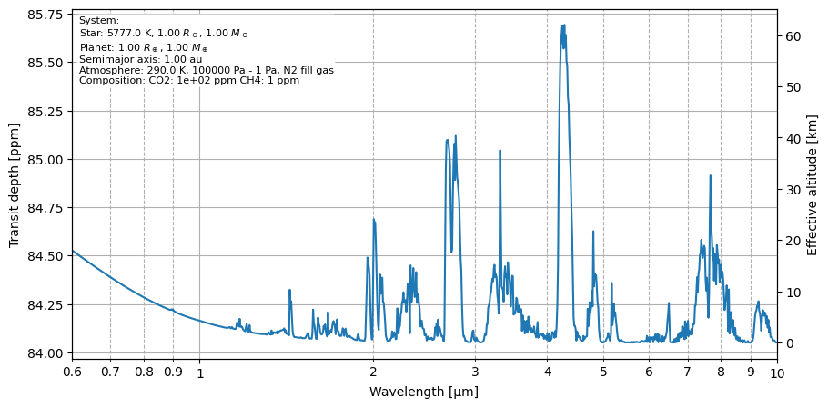
We have automated the spectrum plotting using the routine:
[24]:
fig, ax = system.plot_spectrum(wns,xscale='log')
Studying spectral contributions
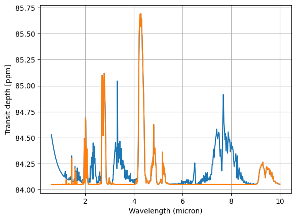
In order to understand a given spectrum you can also calculate all the individual contributions:
[25]:
wns, contributions = system.generate_contributions(wns)
Contributions are also calculated as transit depths. Contributions are given as a dictionary with two keys: Absorption and Rayleigh scattering.
[26]:
plt.plot(wls,spectrum*1e6)
plt.plot(wls,contributions['Absorption']['CO2']*1e6)
plt.grid()
plt.xlabel('Wavelength (micron)')
plt.ylabel('Transit depth [ppm]')
[26]:
Text(0, 0.5, 'Transit depth [ppm]')
We have devised a special method to plot all contributions at once:
[27]:
fig, ax = system.plot_contributions(wns,xscale='log')
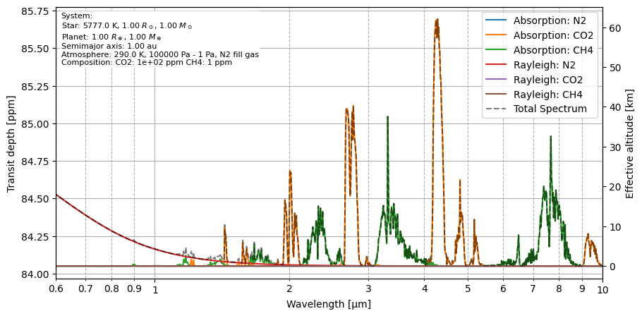
Let’s save this beautiful figure:
[28]:
fig.savefig('resources/contributions-transmission-spectrum.png')
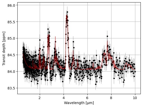
Observations
Once you have a theoretical transmission spectrum you may generate an observed spectrum. In the present version of MultiREx we use a very simplified model for error which is independent of wavelength and signal strength (transit depth). It simply adds a gaussian error to a spectra according to a constant noise which depends on a provided value of the signal-to-noise ratio (SNR).
[29]:
observation = system.generate_observations(wns, snr=10)
observation
Warning: 'params' attribute not found in the DataFrame.
Warning: 'data' attribute not found in the DataFrame. The DataFrame will be considered as having 'data' attribute.
[29]:
| noise | SNR | 10.0 | 9.971877349033692 | 9.943833786417125 | 9.915869089732885 | 9.887983037189068 | 9.860175407617508 | 9.832445980472007 | 9.804794535826622 | ... | 0.6154019907123947 | 0.6136713171735172 | 0.6119455107474266 | 0.6102245577465119 | 0.6085084445216544 | 0.6067971574621212 | 0.6050906829954558 | 0.6033890075873711 | 0.6016921177416427 | 0.6 | |
|---|---|---|---|---|---|---|---|---|---|---|---|---|---|---|---|---|---|---|---|---|---|
| 0 | 1.641670e-07 | 10 | 0.000084 | 0.000084 | 0.000084 | 0.000084 | 0.000084 | 0.000084 | 0.000084 | 0.000084 | ... | 0.000084 | 0.000085 | 0.000085 | 0.000084 | 0.000084 | 0.000084 | 0.000084 | 0.000085 | 0.000085 | 0.000085 |
1 rows × 1002 columns
Observations are returned as a pandas dataframe which is more convenient for manipulation of large sets of spectra. You may obtain wavelengths and transit depths from a dataframe using:
[30]:
noise, wls, spectra = mrex.Physics.df2spectra(observation)
Now you may plot the resulting observed spectrum:
[31]:
plt.plot(wls,spectra[0]*1e6,'k.')
plt.errorbar(wls,spectra[0]*1e6,yerr=noise[0]*1e6,color='k',alpha=0.2)
plt.plot(wls,spectrum*1e6,color='r',alpha=0.5)
plt.grid()
plt.xlabel('Wavelength [μm]')
plt.ylabel('Transit depth [ppm]')
[31]:
Text(0, 0.5, 'Transit depth [ppm]')
Random systems
The superpower of MultiREx is its ability to generate random realizations of a system of star, planet and atmosphere.
Let’s assume for instance that all key parameters of the system components (stellar radius, planetary mass, atmospheric surface pressure, etc.) are physically and statistically independent. If we instantiate a system setting those parameters with a tuple (min,max) the properties of the system will be choosen as a uniformly-deviated random value in the interval [min,max]. See for instance:
[32]:
system=mrex.System(
    star=mrex.Star(
        temperature=(4000,6000),
        radius=(0.5,1.5),
        mass=(0.8,1.2),
    ),
    planet=mrex.Planet(
        radius=(0.5,1.5),
        mass=(0.8,1.2),
        atmosphere=mrex.Atmosphere(
            temperature=(290,310), # in K
            base_pressure=(1e5,10e5), # in Pa
            top_pressure=(1,10), # in Pa
            fill_gas="N2", # the gas that fills the atmosphere
            composition=dict(
                CO2=(-5,-4), # This is the log10(mix-ratio)
                CH4=(-6,-5),
            )
        )
    ),
    sma=(0.5,1)
)
We can check the value of the key properties:
[33]:
print(system.star.mass,
      system.planet.atmosphere.temperature,
      system.planet.atmosphere.base_pressure,
      system.planet.atmosphere.composition,
      system.sma)
0.9244951537961904 301.8283868885127 183797.44925195604 {'CO2': -4.117306805006798, 'CH4': -5.541121549062225} 0.7957096722128167
You may notice that the values are completely random. If you reshuffle the system:
[34]:
system.reshuffle()
The values of the key parameters are entirely different:
[35]:
print(system.star.mass,
      system.planet.atmosphere.temperature,
      system.planet.atmosphere.base_pressure,
      system.planet.atmosphere.composition,
      system.sma)
0.9595311585587656 307.4104332416186 499527.31319022086 {'CO2': -4.618295704432816, 'CH4': -5.33741778980745} 0.9244681334482363
Having a realization of the system with different parameters is like living in a multiverse where everything is the same except for the particular value of the parameters of this system.
Synthesizing spectra in the multiverse
Our last step is to generate a full set of synthetic theoretical and observed spectra for single realizations of the set of key parameters.
[36]:
system.make_tm()
wns = mrex.Physics.wavenumber_grid(wl_min=0.6,wl_max=10,resolution=300)

n_universes = 100
n_observations = 10
data = system.explore_multiverse(wns,snr=10,
                                 n_universes=n_universes,
                                 n_observations=n_observations,
                                 path='/tmp/')

spectra, observations = data.values()
Exploring universes: 100%|██████████| 100/100 [01:01<00:00,  1.63it/s]
/home/jzuluaga/MultiREx-public/multirex/spectra.py:1346: FutureWarning: The behavior of array concatenation with empty entries is deprecated. In a future version, this will no longer exclude empty items when determining the result dtype. To retain the old behavior, exclude the empty entries before the concat operation.
  final_spectra_df = pd.concat([all_header_df, all_spectra_df], axis=1)
Generating observations for 100 spectra...
Let’s analyse the output of this code:
data: A dictionary containing both, spectra and observations.spectra: A dataframe containing the theoretical spectra corresponding to each realization of the system key parameters. The number of rows of this dataframe is equal to then_universesparameter.observations: A dataframe cointaining the observed spectra maden_observationstimes in each parallel universe. The number of rows of this dataframe is equal ton_universes*n_observations.
If you want to compare 3 observed spectra, made at the universe number n we use:
[37]:
n = 5
fig, ax = plt.subplots(figsize=(10,5))
ax.plot(1e4/wns,spectra.data.iloc[n]*1e6,label="True Spectrum",linewidth=0.7)
for i in range(3):
    ax.errorbar(x=1e4/wns,
                 y=observations.data.iloc[n*n_observations+i]*1e6,
                 yerr=observations.params["noise"][n*n_observations+i]*1e6,
                label=f"Observed Spectrum {i}",fmt="o",markersize=2,alpha=0.2)

ax.set_xscale("log")
ax.set_xlabel(r"Wavelength [$\mu$m]")
ax.set_ylabel(r"Transit depth [ppm]")
ax.set_title("Theoretical and observed transmission spectra for different observations of a system")
ax.legend()
ax.margins(x=0)

from matplotlib.ticker import FuncFormatter
formatter = FuncFormatter(lambda y, _: '{:.16g}'.format(y))
ax.xaxis.set_major_formatter(formatter)
formatter = FuncFormatter(lambda y, _: '{:.1g}'.format(y))
ax.xaxis.set_minor_formatter(formatter)

text = ax.text(0.01,0.98,system.__str__(),fontsize=8,verticalalignment='top',transform=ax.transAxes)
text.set_bbox(dict(facecolor='w',alpha=1,edgecolor='w',boxstyle='round,pad=0.1'))

fig.tight_layout()
fig.savefig("resources/synthetic-transmission-spectra.png")
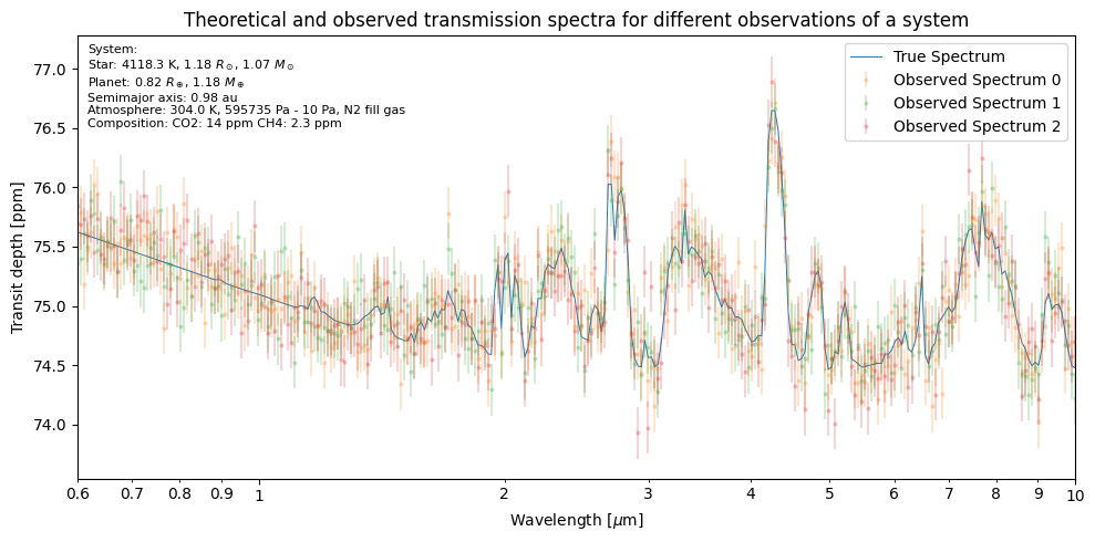
Since in the last command you provided a value for the path variable, a parquet version of the dataframes are stored on disk in the path directory.
WARNING: Be careful when using this options since this files can become extremely large depending on the number of universes and the number of observations per universe.
For more examples and real use-cases of MultiREx see the GitHub repository