MultiREx - Quickstart

Planetary transmission spectra generator

GitHub Repository

Important: Optional Dependencies

To run this notebook fully, you need the optional ggchem dependency. You can install them via:

pip install "multirex[ggchem]"

External dependencies

If you are working in Google Colab use this to install dependencies.

import sys
if 'google.colab' in sys.modules:
    !pip install -Uq multirex
    !mkdir resources/

NOTE: After installing you should reset Colab session before importing the package. This is to avoid an unintended behavior of the package pybtex.

If you have already reset the Colab session, let’s import MultiREx and any other package required for this example:

import multirex as mrex
import numpy as np
import matplotlib.pyplot as plt
import pandas as pd
# This is for developing purposes
%load_ext autoreload
%autoreload 2

Loading MultiREx version 0.3.1

mrex.Util.get_gases(path='tmp/')

Downloading the opacity database to: tmp/

Downloading...
From (original): https://drive.google.com/uc?id=1z7R0hD1IBuYo-nnl7dpE_Ls2337a0uv6
From (redirected): https://drive.google.com/uc?id=1z7R0hD1IBuYo-nnl7dpE_Ls2337a0uv6&confirm=t&uuid=cb0be469-a453-4722-a479-afda1022c6aa
To: c:\Astro\My_repos\MultiREx-public\examples\tmp\opacidades-todas.zip
100%|██████████| 2.12G/2.12G [00:43<00:00, 49.0MB/s]

Once downloaded, the list of available gasses are considerably larger:_

mrex.Util.list_gases()

Available gases in the database:
['CO', 'CH4', 'CO2', 'CH3Cl', 'C2H6', 'DMS', 'N2', 'NO2', 'SO2', 'O3', 'NH3', 'H2O', 'O2', 'HCN']

Creating components of the system

ggchem_params = {
    'metallicity': 1.0,  # Factor de escala para la metalicidad global ([X/H]) respecto al perfil base.
    'selected_elements': ['C','O','H','N','S'], # Lista de elementos a incluir en la red química.
    'ratio_elements': ['C'], # Elementos para los cuales se definirán explícitamente las proporciones (e.g., C/O).
    'abundance_profile': 'earthcrust',  # Perfil de abundancia de referencia (e.g., 'solar' para abundancias solares).
    'ratios_to_O': [0.45],  # Proporciones de los 'ratio_elements' respecto al Oxígeno. Aquí, C/O = 0.54.
    'equilibrium_condensation': True, # Booleano para activar o desactivar la condensación en equilibrio.
    # 'output_gases': ['H2O', 'CO', 'CO2', 'CH4', 'NH3', 'HCN', 'Na', 'K', 'TiO', 'VO'] # Opcional: lista para forzar la salida de gases específicos.
}

system = mrex.System(
    star=mrex.Star(
        temperature=5777,
        radius=1,
        mass=1
    ),
    planet=mrex.Planet(
        radius=1,
        mass=1,
        atmosphere=mrex.Atmosphere(
            temperature=700, # in K
            base_pressure=1e5, # in Pa
            top_pressure=1, # in Pa
            chemistry_type='ggchem', # Especifica 'ggchem' para utilizar el modelo químico GGChem.
            ggchem_params=ggchem_params # Pasa los parámetros de GGChem definidos anteriormente.
        )
    ),
    sma=1
)

The transmission model

Once we have a system we can create the transmission model:

system.make_tm()

Generating a transmission spectrum

In order to create and manipulate a transmission spectrum, we need first to genereta a wave number grid:

wns = mrex.Physics.wavenumber_grid(wl_min=0.6,wl_max=10,resolution=1000)

The corresponding wavelength grid is:

wls = np.sort(1e4/wns)
wls[:10],wls[-10:]

(array([0.6       , 0.60169212, 0.60338901, 0.60509068, 0.60679716,
        0.60850844, 0.61022456, 0.61194551, 0.61367132, 0.61540199]),
 array([ 9.74972472,  9.77722085,  9.80479454,  9.83244598,  9.86017541,
         9.88798304,  9.91586909,  9.94383379,  9.97187735, 10.        ]))

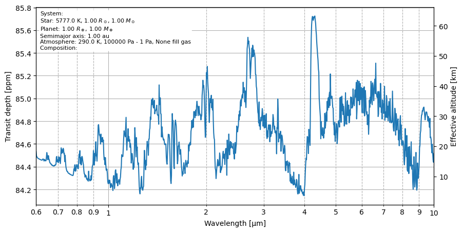
Let’s generate the transmission spectrum:

wns,spectrum = system.generate_spectrum(wns)
wls = 1e4/wns

fig, ax = system.plot_spectrum(wns,xscale='log')

Studying spectral contributions

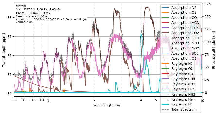
In order to understand a given spectrum you can also calculate all the individual contributions:

wns, contributions = system.generate_contributions(wns)

Contributions are also calculated as transit depths. Contributions are given as a dictionary with two keys: Absorption and Rayleigh scattering.

We have devised a special method to plot all contributions at once:

fig, ax = system.plot_contributions(wns,xscale='log')

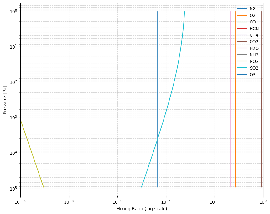
system.plot_mixing_ratio(min_mix=1e-10,
 #list_gases=['O3','O2',"SO2"]
 )

(<Figure size 1000x800 with 1 Axes>,
 <Axes: xlabel='Mixing Ratio (log scale)', ylabel='Pressure [Pa]'>)

Including Collision-Induced Absorption (CIA)

In H2/He dominated atmospheres, Collision-Induced Absorption (CIA) can be a significant source of opacity, especially in the infrared. MultiREx allows you to include CIA easily by specifying the cia parameter in the Atmosphere object.

First, let’s download and configure the CIA data cache using Util.get_CIAs():

import multirex.utils as Util

# This will download the CIA cross sections for H2-H2 and H2-He
# and configure the TauREx cache automatically.
Util.get_CIAs(pairs=['H2-H2', 'H2-He'], path='./cia_data')

Now, let’s recreate our planet’s atmosphere adding the cia parameter, and generate a new transmission model.

# Create atmosphere with GGChem and CIA
atm_cia = mrex.Atmosphere(
    temperature=1500,
    base_pressure=1e6,
    top_pressure=1e-4,
    chemistry_type='ggchem',
    ggchem_params=ggchem_params,
    cia=['H2-H2', 'H2-He']
)

planet_cia = mrex.Planet(radius=1.5, mass=1.0, atmosphere=atm_cia)
system_cia = mrex.System(star=star, planet=planet_cia, sma=0.05)

# Build the new transmission model
system_cia.make_tm()

# Generate the spectrum
wns = mrex.Physics.wavenumber_grid(wl_min=0.3, wl_max=10, resolution=500)
bin_wn_cia, bin_rprs_cia = system_cia.generate_spectrum(wns)

# Plot and compare
import matplotlib.pyplot as plt
plt.figure(figsize=(10, 5))
plt.plot(10000/bin_wn, bin_rprs, label='Without CIA', alpha=0.7)
plt.plot(10000/bin_wn_cia, bin_rprs_cia, label='With CIA', alpha=0.7)
plt.xscale('log')
plt.xlabel('Wavelength [μm]')
plt.ylabel('$(R_p/R_s)^2$')
plt.legend()
plt.show()